Lyapunov functions and related concepts are deeply rooted in mathematics and have various applications in finance, particularly in areas requiring stability analysis, optimization, and dynamic modeling.
Let’s explore each concept and its potential financial application:
Lyapunov Function
Lyapunov functions are used in assessing the stability of financial systems or models.
For instance, in risk management, a Lyapunov function can help determine the stability of a financial market or the risk level of an investment portfolio.
It can indicate whether small disturbances in market conditions or asset prices will die out or escalate.
Lyapunov Stability
This concept is crucial in analyzing the stability of economic models or financial systems.
For example, Lyapunov stability can be applied to study the robustness of financial markets under external shocks, ensuring that the system returns to equilibrium after small perturbations, which is vital in macroeconomic modeling.
Ordinary Differential Equations (ODEs)
ODEs are used to model dynamic systems in finance, such as interest rate models, stock price evolution (e.g., Black-Scholes model), or macroeconomic growth models.
These equations can describe how financial variables evolve over time under various influences.
Control-Lyapunov Function
This concept can be applied in optimal control problems in finance.
For instance, in portfolio optimization, a Control-Lyapunov function can be used to develop strategies that minimize risk while controlling for return, ensuring the portfolio’s stability and performance under different market conditions.
Chetaev Function
Similar to Lyapunov functions, Chetaev functions can be used to analyze the instability in financial systems.
They might be applied in stress testing scenarios where the goal is to understand under what conditions a financial system might become unstable.
Foster’s Theorem
Foster’s theorem, often used in stochastic processes, can be applied to assess the stability of financial systems modeled as Markov processes.
This could be useful in credit risk modeling, where the credit ratings of borrowers evolve as a stochastic process, and the objective is to ensure long-term stability of the credit portfolio.
Lyapunov Optimization
This optimization technique can be used in dynamic resource allocation problems in finance.
For example, in high-frequency trading, Lyapunov optimization can help in making real-time decisions about asset allocation to maximize returns while controlling for risk and maintaining system stability.
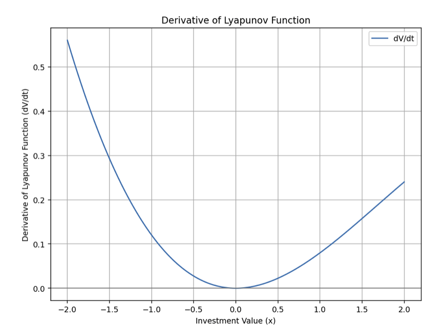
Lyapunov Function in Python
To provide a Python example involving a Lyapunov function in a financial context, let’s consider a simplified scenario where we use a Lyapunov function to assess the stability of a basic financial model. Suppose we have a financial model describing the growth of an investment over time, which can be affected by market volatility.
Let’s define our system with a simple differential equation and then construct a Lyapunov function to assess its stability. The differential equation might represent the growth rate of an investment, and the Lyapunov function will help us determine if the investment’s value will converge to a stable point over time.
Scenario
- Financial Model (Differential Equation):
- Assume the growth of an investment follows the differential equation: , where:
- is the value of the investment.
- and are constants representing linear growth and a quadratic term representing market impact, respectively.
- Assume the growth of an investment follows the differential equation: , where:
- Lyapunov Function:
- We choose a Lyapunov function , a common choice for analyzing stability around the origin.
- Stability Analysis:
- To assess stability, we compute the derivative of along the system trajectories, , and check if it is negative.
Python implementation of a Lyapunov function in a financial context
import numpy as np
import matplotlib.pyplot as plt

# Parameters for the model
a = 0.05 # Linear growth rate
b = 0.01 # Quadratic term for market impact

# Differential equation representing the investment growth
def investment_growth(x):
return a * x - b * x**2

# Lyapunov function
def lyapunov_function(x):
return x**2

# Derivative of the Lyapunov function
def derivative_lyapunov(x):
return 2 * x * investment_growth(x)

# Analyzing stability
x_values = np.linspace(-2, 2, 400)
lyapunov_derivative = derivative_lyapunov(x_values)

# Plotting
plt.figure(figsize=(10, 6))
plt.plot(x_values, lyapunov_derivative, label="dV/dt")
plt.axhline(0, color='grey', lw=1)
plt.title("Derivative of Lyapunov Function")
plt.xlabel("Investment Value (x)")
plt.ylabel("Derivative of Lyapunov Function (dV/dt)")
plt.grid(True)
plt.legend()
plt.show()
FAQs – Lyapunov Functions in Finance
What is a Lyapunov function and how is it applied in financial stability analysis?
A Lyapunov function is a mathematical tool used to determine the stability of a dynamical system.
In finance, it is applied to analyze the stability of various financial models or systems.
By choosing an appropriate Lyapunov function, one can assess whether small disturbances or shocks to a financial system will dissipate over time, indicating stability, or grow, indicating instability.
For example, in risk management, a Lyapunov function can help evaluate the stability of a portfolio’s returns or a financial market’s dynamics.
How does Lyapunov stability differ from other stability concepts in financial models?
Lyapunov stability focuses on the behavior of dynamical systems in response to small perturbations from equilibrium states.
It differs from other stability concepts as it provides a local perspective, examining whether a system, once slightly disturbed, returns to its equilibrium.
Other stability concepts might focus on global stability (behavior over the entire system’s state space) or asymptotic stability (whether the system converges to an equilibrium over time).
Lyapunov stability is particularly useful in financial models for assessing the resilience of equilibrium points to small external shocks.
Can you provide examples of ordinary differential equations commonly used in financial modeling?
Ordinary Differential Equations (ODEs) are widely used in financial modeling to describe the continuous evolution of financial variables over time.
Common examples include:
- The Black-Scholes equation for option pricing, which models the price of a financial derivative.
- Models of interest rate dynamics, such as the Vasicek model, which describes the evolution of interest rates over time.
- Differential equations in macroeconomic models, like the Solow growth model, which describes how output evolves based on capital, labor, and technological progress.
What role does a Control-Lyapunov function play in financial risk management?
A Control-Lyapunov function is used in optimal control problems and can be applied in financial risk management to develop strategies that balance risk and return.
By utilizing a Control-Lyapunov function, financial managers can devise control strategies (like adjusting asset allocations in a portfolio) that ensure the system (such as a portfolio or a financial institution) remains stable and performs optimally under varying market conditions.
How is the Chetaev function used to predict financial market instability?
The Chetaev function, similar to a Lyapunov function but used for assessing instability, can help in predicting conditions under which a financial market might become unstable.
By applying a Chetaev function to a financial model, analysts can identify scenarios or shocks that could lead to unstable market behavior, such as rapid asset price declines or heightened volatility, thus aiding in proactive risk management.
What is Foster’s theorem and how is it relevant in the context of financial stochastic processes?
Foster’s theorem is a result in the theory of stochastic processes, particularly Markov chains, that provides criteria for determining the stability and ergodicity of these processes.
In finance, it’s relevant for models where the state of a system (like credit ratings in a portfolio) evolves as a stochastic process.
Foster’s theorem can help in determining whether such systems will remain stable over time, avoiding undesirable states, which is crucial in areas like credit risk management.
How does Lyapunov optimization aid in portfolio management and asset allocation?
Lyapunov optimization is a technique used to make dynamic decisions in systems with uncertainty.
In portfolio management and asset allocation, it can help in making real-time adjustments to a portfolio, optimizing for factors such as return, risk, and liquidity under varying market conditions.
This technique allows for a disciplined, mathematical approach to balancing risk and reward over time, taking into account both current market conditions and predicted future states.
Can Lyapunov functions be used to analyze the stability of cryptocurrency markets?
Yes, Lyapunov functions can be used to analyze the stability of cryptocurrency markets.
Given the high volatility and dynamic nature of these markets, a Lyapunov function can help assess how small changes in market factors (like regulatory news or technological advancements) could impact market stability.
This is particularly useful in understanding the resilience of cryptocurrencies to shocks and in designing risk management strategies.
How do Lyapunov functions help in understanding the dynamics of interest rate models?
Lyapunov functions can be instrumental in analyzing the stability of interest rate models, which are often dynamic and complex.
By applying a Lyapunov function to these models, one can determine whether the interest rates, under the influence of various economic factors and shocks, will converge to a stable equilibrium or diverge.
This is crucial for long-term financial planning and risk assessment, as stable interest rates are often a key assumption in many financial models and investment strategies.
What are the limitations of using Lyapunov stability in complex financial systems?
The primary limitations of using Lyapunov stability in complex financial systems include:
- Locality: Lyapunov stability is a local concept, often only applicable near equilibrium points. It may not provide information about the system’s behavior far from these points.
- Existence of a Suitable Function: Finding an appropriate Lyapunov function can be challenging, especially for complex or nonlinear financial systems.
- Complexity and Computation: Analyzing Lyapunov stability in high-dimensional or highly nonlinear systems can be computationally intensive and mathematically complex.
- Lack of Universality: Lyapunov stability may not account for all types of market behaviors, especially under extreme conditions or in highly irrational markets.
How is the concept of a Control-Lyapunov function integrated into algorithmic trading strategies?
In algorithmic trading, a Control-Lyapunov function can be integrated to manage risk and optimize trading strategies dynamically.
It helps in formulating control laws that adjust trading actions (like buying, selling, or holding assets) to maintain desired levels of risk and return.
By considering market volatility, trade costs, and other factors, the Control-Lyapunov function aids in devising strategies that ensure profitability while keeping the trading system stable and responsive to market changes.
In what ways can Chetaev functions contribute to the stress testing of financial institutions?
Chetaev functions can be valuable in stress testing financial institutions by identifying potential instability scenarios.
By applying Chetaev functions to different financial models (like those representing asset portfolios, liabilities, or liquidity conditions), institutions can simulate how these models behave under extreme or adverse conditions.
This approach helps in uncovering vulnerabilities and ensuring that the institution remains resilient even in the face of significant financial shocks or stressors.
How is Foster’s theorem applied in credit risk modeling and rating transitions?
In credit risk modeling, Foster’s theorem is used to analyze the behavior of credit rating transitions, which can be modeled as Markov processes.
The theorem provides criteria to ensure that the credit ratings do not persist in a low state (i.e., high default risk) indefinitely.
By applying Foster’s theorem, financial institutions can assess the long-term stability of their credit portfolios, ensuring that they are likely to revert to more favorable states over time and thus mitigating the risk of prolonged exposure to high default risks.
Can Lyapunov optimization be used for real-time decision-making in high-frequency trading?
Yes, Lyapunov optimization is well-suited for real-time decision-making in high-frequency trading.
It allows for the development of algorithms that can quickly adjust trading strategies in response to market fluctuations, ensuring profitability while managing risk.
The optimization technique balances the trade-off between immediate rewards and long-term stability, making it ideal for the fast-paced and often volatile environment of high-frequency trading.
By continuously adjusting positions in response to real-time market data, Lyapunov optimization helps in maintaining optimal portfolio performance.
Conclusion
Each of these applications requires a deep understanding of both the mathematical concepts and their financial implications.
They enable the creation of more robust, stable, and efficient financial models and systems